Using a shapefile to generate a network#
Imports#
Import the required libraries
import opentnsim
print('This notebook has been tested with OpenTNSim version {}'.format(opentnsim.__version__))
This notebook has been tested with OpenTNSim version 1.3.7
# package(s) related to time, space and id
import datetime
import platform
import random
import os
import pathlib

# you need these dependencies (you can get these from anaconda)
# package(s) related to the simulation
import simpy

# spatial libraries
import shapely.geometry
import geopandas as gpd

# package(s) for data handling
import numpy as np
import matplotlib.pyplot as plt

# OpenTNSIM
import opentnsim.graph_module as graph_module
import opentnsim.utils

# Used for making the graph to visualize our problem
import networkx as nx
# Graph location
src_dir = pathlib.Path(opentnsim.__file__).parent.parent
data_path = src_dir / "notebooks" / "Shape-Files"
shape_path = data_path  / "Amsterdam-Canals" / "final_network_v4.shp"
Create graph#
Important:
If you use windows and get the following error “ImportError: read_shp requires OGR: http://www.gdal.org/”, you probably have this issue. Solving it is possible by running the following commands in your terminal (as explained here:
#Create a new virtual environment
conda create -n testgdal -c conda-forge gdal vs2015_runtime=14

#Activate virtual environment
activate testgdal

#Open Jupyter notebook
jupyer notebook
Create a graph from geospatial information#
The process to create a graph from a geospatial dataset is the following:
dataset -> geopandas dataframe -> project to wgs84 -> networkx
This allows you to use all the data formats that geopandas supports. We always use wgs84 to import the graph. That way we can apply our algorithms anywhere in the world.
Dataset to geopandas#
Let’s first convert the data from it’s oringal format to geopandas. Geopandas dataframes are tables with a geospatial column.
# read the file using geopandas
# we need to specify the EPSG code to make sure

gdf = gpd.read_file(shape_path)
# store length in meters before we convert to degrees
gdf['length_m'] = gdf.geometry.length
print(gdf.crs.name)
gdf.head()
Amersfoort / RD New
| edge_id | cost | width | turnaround | turn_aroun | geometry | length_m | |
|---|---|---|---|---|---|---|---|
| 0 | 0.0 | 47.952194 | 50.0 | 0 | NaN | LINESTRING (122153.226 485731.135, 122138.316 ... | 47.952194 |
| 1 | 1.0 | 30.921218 | 50.0 | 0 | NaN | LINESTRING (122138.316 485776.71, 122138.21 48... | 30.921218 |
| 2 | 2.0 | 214.380539 | 13.0 | 0 | NaN | LINESTRING (122129.447 485806.332, 121924.805 ... | 214.380539 |
| 3 | 3.0 | 304.623228 | 13.0 | 0 | NaN | LINESTRING (121187.522 485724.593, 121152.736 ... | 304.623228 |
| 4 | 4.0 | 575.560869 | 13.0 | 0 | NaN | LINESTRING (121758.376 485690.501, 121734.422 ... | 575.560869 |
# this should contain Rijksdriehoek (RD)
gdf_wgs84 = gdf.to_crs('EPSG:4326')
print(gdf_wgs84.crs.name)
gdf.head()
WGS 84
| edge_id | cost | width | turnaround | turn_aroun | geometry | length_m | |
|---|---|---|---|---|---|---|---|
| 0 | 0.0 | 47.952194 | 50.0 | 0 | NaN | LINESTRING (122153.226 485731.135, 122138.316 ... | 47.952194 |
| 1 | 1.0 | 30.921218 | 50.0 | 0 | NaN | LINESTRING (122138.316 485776.71, 122138.21 48... | 30.921218 |
| 2 | 2.0 | 214.380539 | 13.0 | 0 | NaN | LINESTRING (122129.447 485806.332, 121924.805 ... | 214.380539 |
| 3 | 3.0 | 304.623228 | 13.0 | 0 | NaN | LINESTRING (121187.522 485724.593, 121152.736 ... | 304.623228 |
| 4 | 4.0 | 575.560869 | 13.0 | 0 | NaN | LINESTRING (121758.376 485690.501, 121734.422 ... | 575.560869 |
Convert to networkx Graph#
FG = graph_module.gdf_to_nx(gdf_wgs84)
# We want an undirected graph for two-way traffic
FG = FG.to_undirected()
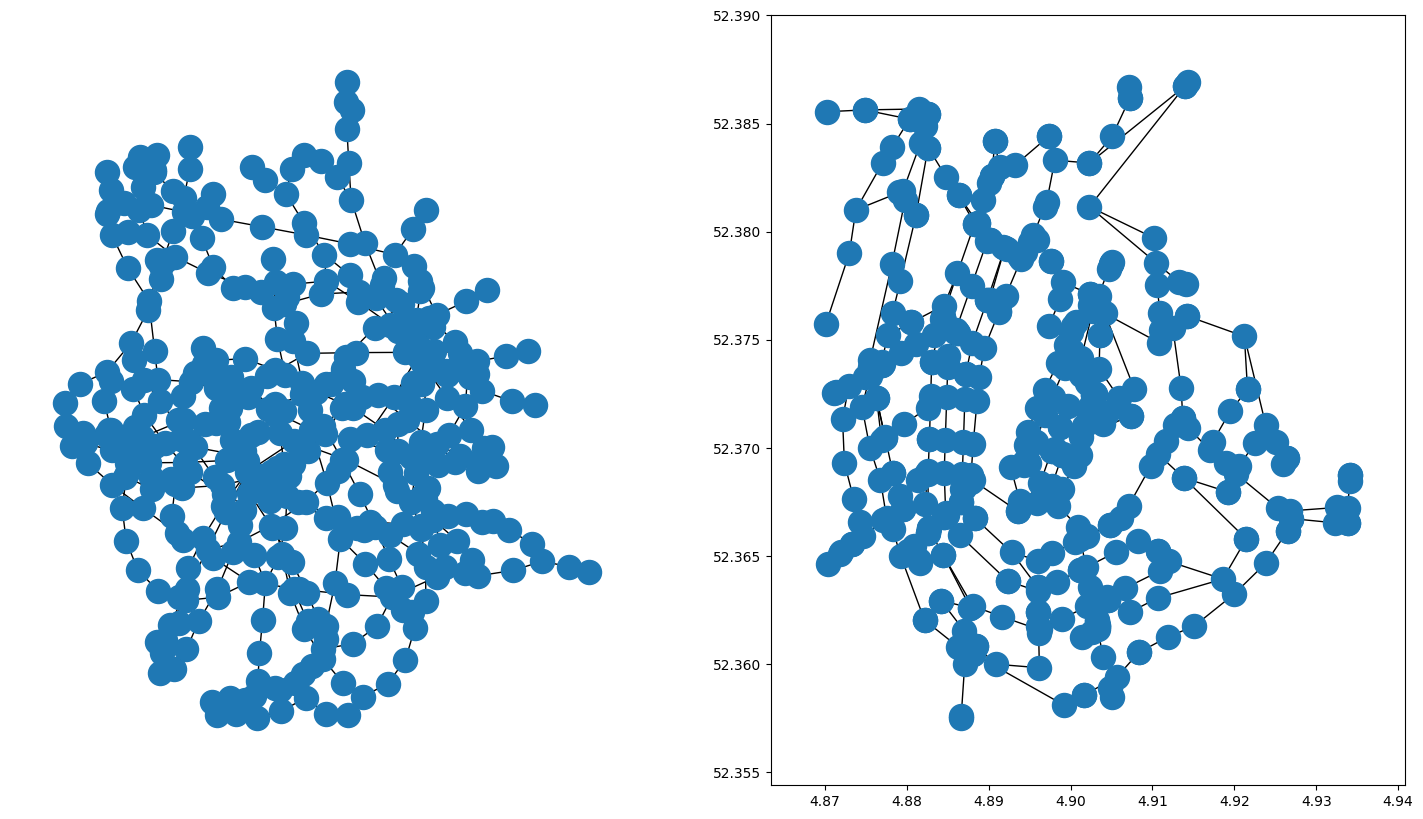
fig, axes = plt.subplots(figsize=(18, 10), ncols=2)
nx.draw(FG, ax=axes[0])
xy = nx.get_node_attributes(FG, 'n')
nx.draw(FG, pos=xy, ax=axes[1])
axes[1].axis('on')
axes[1].tick_params(left=True, bottom=True, labelleft=True, labelbottom=True)
print('The first edge attributes')
print(list(FG.edges.values())[0])
print()
print('The first node attributes')
print(list(FG.nodes.values())[0])
The first edge attributes
{'edge_id': 0.0, 'cost': 47.9521941009, 'width': 50.0, 'turnaround': 0, 'turn_aroun': nan, 'length_m': 47.95219410085968, 'Wkt': 'LINESTRING (4.9050273343119368 52.3584927024455880, 4.9048040135335418 52.3589014100909935)', 'Wkb': b'\x01\x02\x00\x00\x00\x02\x00\x00\x00^lK|\xbf\x9e\x13@\xe2m\xc0\x16\xe3-J@\x17\xaa}\xf1\x84\x9e\x13@ j={\xf0-J@', 'Json': {'type': 'LineString', 'coordinates': ((4.905027334311937, 52.35849270244559), (4.904804013533542, 52.35890141009099))}, 'e': [(4.905027334311937, 52.35849270244559), (4.904804013533542, 52.35890141009099)]}

The first node attributes
{'Wkt': 'POINT (4.9050273343119368 52.3584927024455880)', 'Wkb': b'\x01\x01\x00\x00\x00^lK|\xbf\x9e\x13@\xe2m\xc0\x16\xe3-J@', 'Json': {'type': 'Point', 'coordinates': (4.905027334311937, 52.35849270244559)}, 'n': (4.905027334311937, 52.35849270244559)}
Show on a map#
We can also generate a real map. For this we have to step back to pandas, to geopandas and then to ipyleaflet.
networkx -> pandas -> geopandas -> ipyleaflet
df_edges = nx.to_pandas_edgelist(FG)
# generate a geodataframe from the edges, using the Wkt to reconstruct the geometry
gdf_edges = gpd.GeoDataFrame(df_edges, geometry=df_edges['Wkt'].apply(shapely.wkt.loads))
gdf_edges.head()
| source | target | width | turnaround | Json | length_m | e | cost | Wkb | Wkt | edge_id | turn_aroun | geometry | |
|---|---|---|---|---|---|---|---|---|---|---|---|---|---|
| 0 | (4.905027334311937, 52.35849270244559) | (4.904804013533542, 52.35890141009099) | 50.0 | 0 | {'type': 'LineString', 'coordinates': ((4.9050... | 47.952194 | [(4.905027334311937, 52.35849270244559), (4.90... | 47.952194 | b'\x01\x02\x00\x00\x00\x02\x00\x00\x00^lK|\xbf... | LINESTRING (4.9050273343119368 52.358492702445... | 0.0 | NaN | LINESTRING (4.90503 52.35849, 4.9048 52.3589) |
| 1 | (4.904804013533542, 52.35890141009099) | (4.904670934508645, 52.35916710216342) | 50.0 | 0 | {'type': 'LineString', 'coordinates': ((4.9048... | 30.921218 | [(4.904804013533542, 52.35890141009099), (4.90... | 30.921218 | b'\x01\x02\x00\x00\x00\x03\x00\x00\x00\x17\xaa... | LINESTRING (4.9048040135335418 52.358901410090... | 1.0 | NaN | LINESTRING (4.9048 52.3589, 4.9048 52.3589, 4.... |
| 2 | (4.904670934508645, 52.35916710216342) | (4.901673214470882, 52.35858070824794) | 13.0 | 0 | {'type': 'LineString', 'coordinates': ((4.9046... | 214.380539 | [(4.904670934508645, 52.35916710216342), (4.90... | 214.380539 | b'\x01\x02\x00\x00\x00\x02\x00\x00\x00\xf1l\xb... | LINESTRING (4.9046709345086450 52.359167102163... | 2.0 | NaN | LINESTRING (4.90467 52.35917, 4.90167 52.35858) |
| 3 | (4.904670934508645, 52.35916710216342) | (4.903965447805071, 52.36034084357929) | 50.0 | 0 | {'type': 'LineString', 'coordinates': ((4.9046... | 139.210726 | [(4.904670934508645, 52.35916710216342), (4.90... | 139.210726 | b'\x01\x02\x00\x00\x00\x03\x00\x00\x00\xf1l\xb... | LINESTRING (4.9046709345086450 52.359167102163... | 14.0 | NaN | LINESTRING (4.90467 52.35917, 4.90408 52.36011... |
| 4 | (4.904670934508645, 52.35916710216342) | (4.905708508467728, 52.35943195740624) | 13.0 | 0 | {'type': 'LineString', 'coordinates': ((4.9057... | 76.578295 | [(4.905708508467728, 52.35943195740624), (4.90... | 76.578295 | b'\x01\x02\x00\x00\x00\x02\x00\x00\x00\xb3O\x1... | LINESTRING (4.9057085084677281 52.359431957406... | 134.0 | NaN | LINESTRING (4.90571 52.35943, 4.90467 52.35917) |
import ipyleaflet
m = ipyleaflet.Map(
    basemap=ipyleaflet.basemap_to_tiles(ipyleaflet.basemaps.OpenStreetMap.Mapnik),
    center=(52.37, 4.90),
    zoom=13
    )

style = {'color': 'purple', 'opacity':0.5, 'weight':5}
# show the geometry
geo_data = ipyleaflet.GeoData(geo_dataframe=gdf_edges[['geometry']], style=style)

m.add_layer(geo_data)
m