Comparing alternative routes#
In this notebook, we show how to setup a simple transport network and compare different routes to the same destination
We take the following steps:
1. Imports#
We start with importing required libraries
# package(s) used for creating and geo-locating the graph
import networkx as nx
import shapely.geometry
import pyproj

# package(s) related to the simulation (creating the vessel, running the simulation)
import datetime, time
import simpy
import opentnsim

# package(s) needed for inspecting the output
import pandas as pd

# package(s) needed for plotting
import matplotlib.pyplot as plt

print('This notebook is executed with OpenTNSim version {}'.format(opentnsim.__version__))
This notebook is executed with OpenTNSim version 1.3.7
2. Create vessel#
We start with creating a vessel class. We call this class a Vessel, and add a number of OpenTNSim mix-ins to this class. Each mix-in requires certain input parameters.
The following mix-ins are sufficient to create a vessel for our problem:
Identifiable - allows to give the vessel a name and a random ID,
Movable - allows the vessel to move, with a fixed speed, while logging this activity,
Movable in turn relies on the mix-ins: Locatable, Routeable, and Log
# make your preferred Vessel class out of available mix-ins.
Vessel = type('Vessel',
              (opentnsim.core.Identifiable,
               opentnsim.core.Movable), {})
# create a dict with all important settings
data_vessel = {"env": None,          # needed for simpy simulation
               "name": 'Vessel 1',   # required by Identifiable
               "geometry": None,     # required by Locatable
               "route": None,        # required by Routeable
               "v": 1}               # required by Movable
3. Create graph#
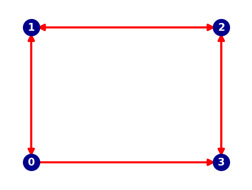
Next we create a 1D network (a graph) along which the vessel can move. A graph is made of nodes (blue dots in the plot below) and edges (red arrows between the nodes in the plot below). We use the python package networkx to do this.
For this example, we construct a network of 4 nodes linked by 7 edges. The edges are made bi-directional to allow for two-way traffic, exept for one edge. This enables us to select two different routes between two nodes.
# specify a number of coordinates along your route (coords are specified in world coordinates: lon, lat)
coords = [
    [0,0],
    [0,0.1],
    [0.1,0.1],
    [0.1,0]]
# make your preferred Site class out of available mix-ins.
Node = type('Site', (opentnsim.core.Identifiable, opentnsim.core.Locatable), {})

# create a list of nodes
nodes = []
for index, coord in enumerate(coords):
    data_node = {"name": str(index), "geometry": shapely.geometry.Point(coord[0], coord[1])}
    nodes.append(Node(**data_node))
# create a graph
FG = nx.DiGraph()

# add nodes
for node in nodes:
    FG.add_node(node.name, geometry = node.geometry)

# add edges
path = [
        [nodes[0], nodes[3]], # From node 0 to node 3 - so from node 0 to node 3 is one-way traffic
        [nodes[0], nodes[1]], # From node 0 to node 1 - all other edges are two-way traffic
        [nodes[1], nodes[0]], # From node 1 to node 0
        [nodes[1], nodes[2]], # From node 1 to node 2
        [nodes[2], nodes[1]], # From node 2 to node 1
        [nodes[2], nodes[3]], # From node 2 to node 3
        [nodes[3], nodes[2]], # From node 3 to node 2
       ]

for edge in path:
    FG.add_edge(edge[0].name, edge[1].name, weight = 1)
# create a positions dict for the purpose of plotting
positions = {}
for node in FG.nodes:
    positions[node] = (FG.nodes[node]['geometry'].x, FG.nodes[node]['geometry'].y)
# collect node labels
labels = {}
for node in FG.nodes:
    labels[node] = node
# draw edges, nodes and labels.
nx.draw_networkx_edges(FG,  pos=positions, width=3, edge_color="red", alpha=1, arrowsize=20)
nx.draw_networkx_nodes(FG,  pos=positions, node_color="darkblue", node_size=600)
nx.draw_networkx_labels(FG, pos=positions, labels=labels, font_size=15, font_weight='bold', font_color="white")

plt.axis("off")
plt.show()
# To show that moving from Node 4 to Node 1 is not possible
print("From 0 to 3: {} edge".format(nx.shortest_path_length(FG, "0", "3")))
print("From 3 to 0: {} edges".format(nx.shortest_path_length(FG, "3", "0")))
From 0 to 3: 1 edge
From 3 to 0: 3 edges
4. Run simulation(s)#
def calculate_distance(orig, dest):
    """method to calculate the greater circle distance in meters from WGS84 lon, lat coordinates"""

    wgs84 = pyproj.Geod(ellps='WGS84')
    distance = wgs84.inv(orig.x, orig.y,
                         dest.x, dest.y)[2]

    return distance
def calculate_distance_along_path(FG, path):
    """method to calculate the greater circle distance along path in meters from WGS84 lon, lat coordinates"""

    distance_path = 0

    for node in enumerate(path[:-1]):
        orig = nx.get_node_attributes(FG, "geometry")[path[node[0]]]
        dest = nx.get_node_attributes(FG, "geometry")[path[node[0]+1]]
        distance_path += calculate_distance(orig, dest)

        if node[0] + 2 == len(path):
                    break

    return distance_path
def start(env, vessel):
    """method that defines the simulation (keep moving along the path until its end point is reached)"""
    while True:
        yield from vessel.move()

        if vessel.geometry == nx.get_node_attributes(FG, "geometry")[vessel.route[-1]]:
            break
# first simulation is from Node 1 to Node 4
path_1 = nx.dijkstra_path(FG, "0", "3")

# second simulation is from Node 4 to Node 1
path_2 = nx.dijkstra_path(FG, "3", "0")

# collect paths in list
paths = [path_1, path_2]
# run a simulation for each path in the list
for path in enumerate(paths):

    # Start simpy environment
    simulation_start = datetime.datetime.now()
    env = simpy.Environment(initial_time = time.mktime(simulation_start.timetuple()))
    env.epoch = time.mktime(simulation_start.timetuple())

    # Add graph to environment
    env.FG = FG

    # create the transport processing resource
    vessel = Vessel(**data_vessel)

    # Add environment and path to the vessel
    vessel.env = env
    vessel.route = path[1]
    vessel.geometry = FG.nodes[path[1][0]]['geometry']

    # Start the simulation
    env.process(start(env, vessel))
    env.run()

    df = pd.DataFrame.from_dict(vessel.log)
    display(df)

    print("Simulation of path {} took {:.1f} seconds".format(path[0] + 1, (env.now - simulation_start.timestamp())))

    print("Distance of path {} is {:.1f} meters".format(path[0] + 1, calculate_distance_along_path(FG, path[1])))
| Timestamp | |
|---|---|
| 0 | 2025-06-12 14:55:13.000000 |
| 1 | 2025-06-12 18:00:44.949079 |
Simulation of path 1 took 11131.1 seconds
Distance of path 1 is 11131.9 meters
| Timestamp | |
|---|---|
| 0 | 2025-06-12 14:55:13.000000 |
| 1 | 2025-06-12 17:59:30.427695 |
| 2 | 2025-06-12 17:59:30.427695 |
| 3 | 2025-06-12 21:05:02.359933 |
| 4 | 2025-06-12 21:05:02.359933 |
| 5 | 2025-06-13 00:09:19.787627 |
Simulation of path 2 took 33245.9 seconds
Distance of path 2 is 33246.8 meters
5. Inspect output#
df = pd.DataFrame.from_dict(vessel.log)
df
| Timestamp | |
|---|---|
| 0 | 2025-06-12 14:55:13.000000 |
| 1 | 2025-06-12 17:59:30.427695 |
| 2 | 2025-06-12 17:59:30.427695 |
| 3 | 2025-06-12 21:05:02.359933 |
| 4 | 2025-06-12 21:05:02.359933 |
| 5 | 2025-06-13 00:09:19.787627 |